Getting Started with Imfit: Tutorial
Contents:
Preliminaries
To get started with Imfit, you need to download the pre-compiled binary distribution for your platform (Mac or Linux), or else download and compile the source code; links to both can be found on the main imfit page. Notes on how to compile the source code can be found in the Imfit documentation.
In both the binary-only and source-code distributions, there is a subdirectory called “examples”, which has some images we’ll be using in this tutorial – ic3478rss_256.fits, ic3478rss_256_mask.fits, and psf_moffat_51.fits – as well as some configuration files (names starting with “config_”). You can go ahead and work in the examples subdirectory, or copy the files there to another directory and work there.
If you want to download just the examples directory and its files, you can find it here.
Fitting Your First Image
Imfit requires, as a minimum, two things:
An image in FITS format containing the data to be fit;
A configuration file describing the model you want to fit to the data.
So to start off, we’ll try fitting the image file ic3478rss_256.fits (a 256 x 256-pixel cutout from a DR7 SDSS r-band image of the dwarf elliptical galaxy IC 3478) with a simple exponential model, which is described in the configuration file config_exponential_ic3478_256.dat. To do the fit, just type (all on one line):
imfit ic3478rss_256.fits -c config_exponential_ic3478_256.dat
  --sky=130.14
The --sky=130.14 is a note to Imfit that the image had a background
sky level of 130.14 counts/pixel which was previously subtracted; if we
don’t include this, Imfit will get confused by the fact that some of the
pixels in the image have slightly negative values. (Note that you can
use = or a space to connect an option with its argument on the
command line.)
(Note that, as is normal for Unix-style commands, all invocations of
imfit should be entered as a single line, even though in this and
some of the other examples it’s displayed on two or more lines to fit
the web page better.)
Imfit will print some preliminary information, confirming which files
are being used, the size of the image being fit, the image functions
used in the model, and so forth. It will then call the minimization
routine, which prints a minimal set of updates for each iteration. At
the end, a summary of the fit is printed (final χ2, etc.), along with
the best-fitting parameters of the model and some crude estimates of the
uncertainties for each parameter. These parameters are also saved in a
text file: “bestfit_parameters_imfit.dat”, which includes a record of
how imfit was called and a short summary of the fit. (You can specify a
different name for this output file via the --save-params option.)
Reduced Chi^2 = 0.450366
AIC = 29524.514967, BIC = 29579.055814

X0      128.8530 # +/- 0.0517
Y0      129.1035 # +/- 0.0633
FUNCTION Exponential
PA      19.7364 # +/- 0.467417
ell     0.231428 # +/- 0.00333939
I_0     315.173 # +/- 1.33252
h       20.5726 # +/- 0.0748152
Congratulations; you’ve fit your first image!
Inspecting the Fit: Model Images and Residuals
So what kind of fit did we get, and how good was it? When you run imfit,
you can tell it to save the best-fitting model image, and the residual
image (data - model) as well, using the --save-model and
--save-residual commandline options:
imfit ic3478rss_256.fits -c config_exponential_ic3478_256.dat
  --sky=130.14 --save-model=model.fits --save-residual=resid.fits
These are FITS files with the same dimensions as the data image.
If you look at the residual image (below, right), you can see it’s systematically bright in the center, with an oval region of negative pixels outside. This is a pretty good indication that the exponential model isn’t actually a good match to the data, something we’ll try to address in a bit.
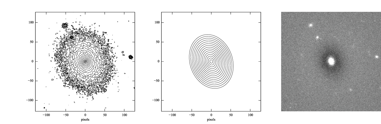
Figure 1: log-scaled isophotes for original SDSS image (left) and best-fitting exponential model (middle), along with linear-scaled residual image (data - model, right).
Generating model images with makeimage
You can also generate a copy of the model image using the “makeimage” program which comes with imfit; it can take a best-fit parameter file produced by imfit as its own input. To run makeimage, you need:
An input configuration file;
Some specification for the size of the output image (this can be included in the configuration file, if you wish).
To run makeimage, you can type
makeimage bestfit_parameters_imfit.dat --refimage=ic3478rss_256.fits
This tells makeimage to make an image with the same dimensions as the
“reference image” (ic3478rss_256.fits, in this case). You can also use
the commandline parameters --ncols and --nrows to directly
specify the output image size, or you can edit the input configuration
file so it specifies the image size there (see the main documentation).
By default, this saves the model image using the filename “model.fits”;
you can use the -o commandline parameter to specify your own name
for the outer file.
Better Fits: Telling Imfit the Truth About the Image
Leaving aside the question of mismatches between an exponential model and the actual galaxy, this isn’t the best possible fit yet for our model. (You may have noticed that imfit reported a reduced χ2 value of ~ 0.45, which is a sign something odd is going on.) For one thing, we’ve deceived imfit about the nature of the data. The default χ2 minimization process that imfit uses is based on the Gaussian approximation to Poisson statistics, and assumes that the pixel values in the image are detected photoelectrons (or N-body particles, or something else that obeys Poisson statistics). In reality, our image deviates from this ideal in three ways:
There was a sky background that was previously subtracted from the image;
The pixel values are counts (ADUs), not detected photoelectrons;
The image has some Gaussian read noise.
To fix this, we can tell imfit three things:
The original background level (which we’re already doing, via the
--skyoption);The A/D gain in electrons/count, via the
--gainoption;The read noise value (in electrons), via the
--readnoiseoption
In the case of this SDSS image, the corresponding tsField FITS table (from the SDSS DR7 archive) has information about the A/D gain and the read noise (or “dark variance”) and tells us that the gain and read noise are 4.725 and 4.3 electrons, respectively, for the r-band image.
So we can re-run the fit with the following command:
imfit ic3478rss_256.fits -c config_exponential_ic3478_256.dat
  --sky=130.14 --gain=4.725 --readnoise=4.3
Now the reduced χ2 is about 2.1, which isn’t necessarily that good, but is at least statistically plausible!
Reduced Chi^2 = 2.082564
AIC = 136482.400611, BIC = 136536.941458

X0      128.8540 # +/- 0.0239
Y0      129.1028 # +/- 0.0293
FUNCTION Exponential
PA      19.7266 # +/- 0.217212
ell     0.23152 # +/- 0.00155236
I_0     316.313 # +/- 0.619616
h        20.522 # +/- 0.0346742
Better Fits: Masking
If you look at the image (e.g., with SAOimage DS9 or another FITS-displaying program), you can see features that most likely aren’t part of the galaxy – for example, there are certainly three (and possibly five) distinct, small objects near the galaxy which are probably foreground stars or background galaxies. Since they’re relatively bright compared to the outer parts of the galaxy, they will bias the fit.
To prevent this from happening, you can mask out parts of an image. This is done with a separate mask image: an image of the same size as the data, but with pixel values = 0 for all the “good” pixels and >= 1 for all the “bad” pixels (i.e., those pixels you want Imfit to ignore).
The file ic3478rss_256_mask.fits in the examples directory is a mask
image. You can use it in the fit with the “--mask” option:
imfit ic3478rss_256.fits -c config_exponential_ic3478_256.dat
  --mask ic3478rss_256_mask.fits --sky=130.14 --gain=4.725
  --readnoise=4.3
(Again, note that options can be linked to their targets with “=” or with just a space, whichever make more sense to you.)
The reduced χ2 is slightly smaller; in addition, the position angle, ellipticity, and scale length of the best-fitting model have changed slightly (the smaller scale length is because imfit is no longer trying to account for the excess light from the other sources by radially stretching the exponential).
Reduced Chi^2 = 1.964467
AIC = 124602.443320, BIC = 124656.787960

X0      128.8793 # +/- 0.0237
Y0      129.0589 # +/- 0.0289
FUNCTION Exponential
PA      18.7492 # +/- 0.23086
ell     0.220646 # +/- 0.00159077
I_0     321.631 # +/- 0.634224
h       20.0684 # +/- 0.034584
Better Fits: Trying Different Models
As noted above, it looks like the exponential model is not a good match
to the galaxy. You can see the available model components (“image
functions”) by calling imfit with the --list-functions option:
imfit --list-functions
You can also see the full set of parameters for each image function
using the --list-parameters option:
imfit --list-parameters
A model fit to an image can consist of multiple image functions (and multiple instances of each image function), but for now let’s just try a Sérsic function with elliptical isophotes. This is encoded in the “config_sersic_ic3478_256.dat” file.
imfit ic3478rss_256.fits -c config_sersic_ic3478_256.dat
  --mask ic3478rss_256_mask.fits --gain=4.725 --readnoise=4.3
  --sky=130.14
The result is a significantly better fit:
Reduced Chi^2 = 1.055366
AIC = 66946.393806, BIC = 67009.795665

X0      128.9321 # +/- 0.0130
Y0      129.0983 # +/- 0.0155
FUNCTION Sersic
PA      19.0449 # +/- 0.247618
ell     0.221656 # +/- 0.00171861
n        2.3108 # +/- 0.00818546
I_e     22.1351 # +/- 0.163568
r_e     56.2217 # +/- 0.256568
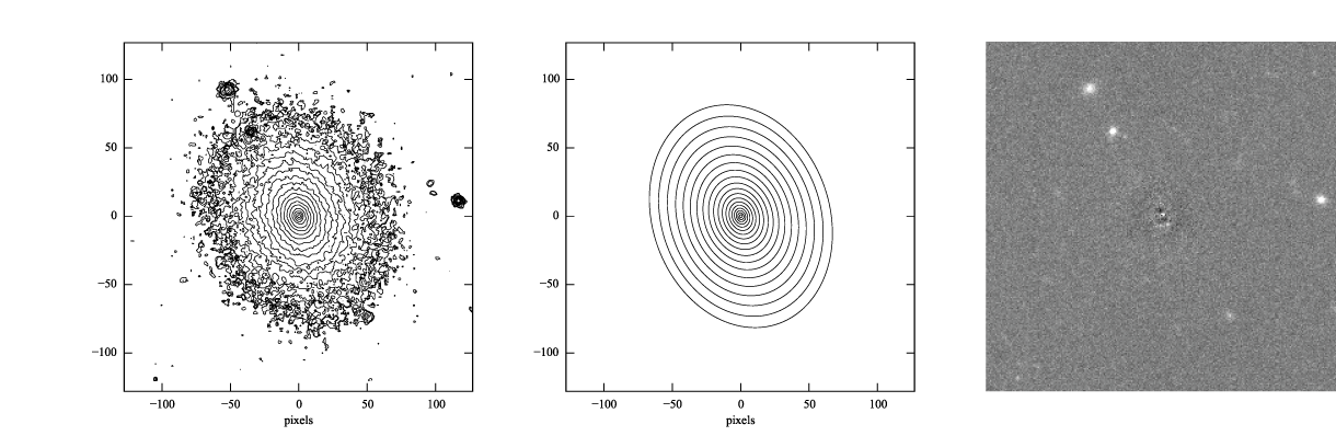
Figure 2: log-scaled isophotes for original SDSS image (left) and best-fitting Sérsic model (middle), along with linear-scaled residual image (data - model, right). Note that the residuals are much improved over the residuals for the exponential model (Figure 1).
This is clearly a much better fit!
More Correct Fits: PSF Convolution
Astronomical images obtained with telescopes are almost always affected by telescope optics, atmospheric seeing, and so forth, so that the actual recorded image – what we’re trying to model – is really the convolution of an idealized “true” image with a point-spread function (PSF).
You can simulate this process in Imfit by providing a PSF image in FITS
format, using the --psf option. This can be any square, centered
image, based on observed stellar PSFs, produced by telescope modeling
software, etc. Imfit will then convolve the internally generated model
image with the PSF image before comparing the model with the data.
Here, we use a pre-generated 51 x 51-pixel PSF image which approximates the seeing in the SDSS image using a circular Moffat function:
imfit ic3478rss_256.fits -c config_sersic_ic3478_256.dat
  --mask ic3478rss_256_mask.fits --gain=4.725 --readnoise=4.3
  --sky=130.14 --psf psf_moffat_51.fits

Reduced Chi^2 = 1.074154
AIC = 68137.906037, BIC = 68201.307896

X0      128.9174 # +/- 0.0147
Y0      129.0800 # +/- 0.0176
FUNCTION Sersic
PA      19.0576 # +/- 0.247209
ell     0.227617 # +/- 0.00175711
n       2.48051 # +/- 0.00983808
I_e     19.9097 # +/- 0.169477
r_e     59.5241 # +/- 0.309487

Figure 3: log-scaled isophotes for original SDSS image (left) and best-fitting, PSF-convolved Sérsic model (middle), along with linear-scaled residual image (data - model, right).
The residuals for the PSF-convolved fit (above right) are systematically somewhat worse than without the PSF (compare with Figure 2): there is a small central excess and a surrounding negative-pixel “moat”. So the galaxy is probably a bit more complicated than just a single Sérsic function can accomodate. (In fact, Janz et al. 2014, working with a higher-resolution and higher-S/N H-band image, found that a Sérsic + exponential model is a better fit for this galaxy than just a Sérsic function by itself.)
Makeimage and PSF images
Makeimage can be used with PSF images to generate properly convolved
model images, using the same --psf option that imfit uses. E.g.
makeimage bestfit_parameters_imfit.dat --refimage=ic3478rss_256.fits
  --psf=psf_moffat_51.fits
Makeimage can also be used to generate PSF images; in fact, the PSF
image we used above was generated using the
“config_makeimage_moffat_psf.dat” configuration file, which is included
in the examples subdirectory (note that this file includes directives
specifying the size of the output image, so the --refimage option
isn’t necessary in this case). A model PSF image can be constructed
using any combination of the image functions that imfit and makeimage
know about – Gaussian, Moffat, the sum of Gaussians and Moffats, etc.
Chi-Squared and All That: Using Different Fit Statistics
Fitting a model to an image involves some assumptions about the underlying statistical model that generated your data – i.e., what kind of statistical distributions the individual pixel values are drawn from. This in turn affects how the “fit statistic” – the quantity you are trying to minimize in order to get the best fit – is calculated.
By default, imfit uses a “data-based” χ2 approach, which assumes that individual pixel values are drawn from the Gaussian approximation of a Poisson distribution. To compare a model pixel value to the data value, we assume that the Gaussian distribution has a mean equal to the model value, with the dispersion equal the square root of the data value. (If you provide a read-noise value, this is added in quadrature to the data-based dispersion.)
One alternative is to take the dispersion from the square root of the
(current) model value, which you can do with the --model-errors
flag:
imfit ic3478rss_256.fits -c config_sersic_ic3478_256.dat
  --mask ic3478rss_256_mask.fits --gain=4.725 --readnoise=4.3
  --sky=130.14 --psf psf_moffat_51.fits --model-errors

Reduced Chi^2 = 1.075389
AIC = 68216.271136, BIC = 68279.672995

X0      128.9250 # +/- 0.0127
Y0      129.0750 # +/- 0.0171
FUNCTION Sersic
PA      19.0862 # +/- 0.247458
ell     0.227161 # +/- 0.00175713
n       2.59104 # +/- 0.0111591
I_e     17.9857 # +/- 0.167361
r_e     63.6443 # +/- 0.360108
The result is not dramatically different, though both n and r_e are slightly larger and I_e is slightly smaller; this is expected due to the differing biases which apply to the data-based and model-based approaches (see Erwin 2015 and references therein).
You can also tell imfit to use an external “noise” or “error” map – an
image whose pixel value are standard deviations, perhaps produced by a
data pipeline. In this case, you use the --noise option to specify
the corresponding FITS file. (If your noise/error map has units of
variance, you can add the --errors-are-variances flag to tell
imfit this.)
Finally, you can abandon the χ2 Gaussian statistical model entirely and
assume that your data comes from a pure Poisson process (rather than the
Gaussian approximation of one). This involves a “Poisson
maximum-likelihood ratio” (Poisson MLR) approach, and is especially
appropriate for data with very low counts per pixel, where the Gaussian
approximation really breaks down. Imfit allows you to do with the
--poisson-mlr flag (or just --mlr for short):
imfit ic3478rss_256.fits -c config_sersic_ic3478_256.dat
  --mask ic3478rss_256_mask.fits --gain=4.725 --sky=130.14
  --psf psf_moffat_51.fits --mlr

Reduced Chi^2 equivalent = 1.104470
AIC = 70060.584150, BIC = 70123.986009

X0      128.9218 # +/- 0.0146
Y0      129.0796 # +/- 0.0173
FUNCTION Sersic
PA      19.0826 # +/- 0.244875
ell     0.227176 # +/- 0.00173874
n       2.55157 # +/- 0.00999606
I_e     18.6469 # +/- 0.162048
r_e     62.1518 # +/- 0.331032
(Note that we leave off the --readnoise option, because the
pure-Poisson approach cannot handle separate read-noise components. In
most cases, this be done without affecting the fit in any significant
way.)
The result is a fit which is in between the two χ2 alternatives, though closer to the model-based approach. (Again, this is consistent with what we would expect from the different statistical models being used, with the pure-Poisson approach being the most unbiased.)
(See Erwin 2015 for more on the statistical background and the corresponding biases.)
Parameter Uncertainties and Correlations: Bootstrap and MCMC
As you probably noticed, part of the output of imfit is a set of 1-sigma parameter uncertainties for each fitted parameter in the model. These are automatically generated when using the default (Levenberg-Marquardt) minimizer. They’re not usually all that accurate, they assume the uncertainties are all symmetric, and they don’t provide any information about possible correlations or anti-correlations between different parameter values.
If you would like a better picture of what the parameter uncertainties and possible correlations are like, there are two options: one fast but noisy, the other slow but detailed:
Boootstrap resampling: This involves generating a new version of the data image by sampling from the original image with replacement (ignoring masked pixels) and re-running the fit. Do this several hundred (or ideally several thousand) times, and you get a distribution of parameter values that can approximate the likelihood (e.g., the χ2).
Markov chain Monte Carlo (MCMC) analysis: This involves computing Markov chains consisting of sequences of sets of parameter values. After an initial “burn-in” period, the distribution of points in parameter space represented by a chain should converge to something proportional to the likelihood. (The particular algorithm used by Imfit actually runs multiple chains in parallel.)
Bootstrap Resampling Example
To save time, we’ll use the model without PSF convolution (you can of course use PSF convolution with bootstrap resampling; it will just take longer):
imfit ic3478rss_256.fits -c config_sersic_ic3478_256.dat
  --mask ic3478rss_256_mask.fits --gain=4.725 --readnoise=4.3
  --sky=130.14 --bootstrap 500 --save-bootstrap=bootstrap_output.dat
This will do the fit as before, print the result, and then start doing 500 rounds of bootstrap resampling and fits to the resampled data. When it’s done (this takes about 30 seconds on a 2012 MacBook Pro with a quad-core CPU) it will print out a summary of the best-fit parameter values and their uncertainties; it will also save all 500 sets of parameter values in the file bootstrap_output.dat.
This file has one column per parameter; the column names are the
parameters with numbers appended (e.g., X0_1, n_1) to make it
possible to distinguish different parameters when multiple versions of
the same function, or just multiple functions that have the same
parameter names, are used in the model. (I.e., all parameters for the
first function will have _1 appended, all parameters from the second
will have _2 appended, etc.)
In the python/ subdirectory of the main Imfit package there are a
couple of Python modules: imfit_funcs.py and imfit.py. The latter has a
simple function to read in the bootstrap-resampling output file
(imfit.GetBootstrapOutput), which will return a list of parameter
names and a 2D Numpy array with the full set of parameter values.
There are many possible ways of analyzing the bootstrap-resampling
output. One thing you can do, if the model is not too complicated, is
make a scatterplot matrix (a.k.a. corner plot) of the parameters. The
Python package corner.py
can be used for this; here’s a quick-and-dirty example that also uses
the imfit.GetBootstrapOutput function:
>>> import imfit, corner

>>> columnNames, bootstrapResults =
    imfit.GetBootstrapOutput("bootstrap_output.dat")
>>> corner.corner(bootstrapResults, labels=columnNames)
The result is shown below.
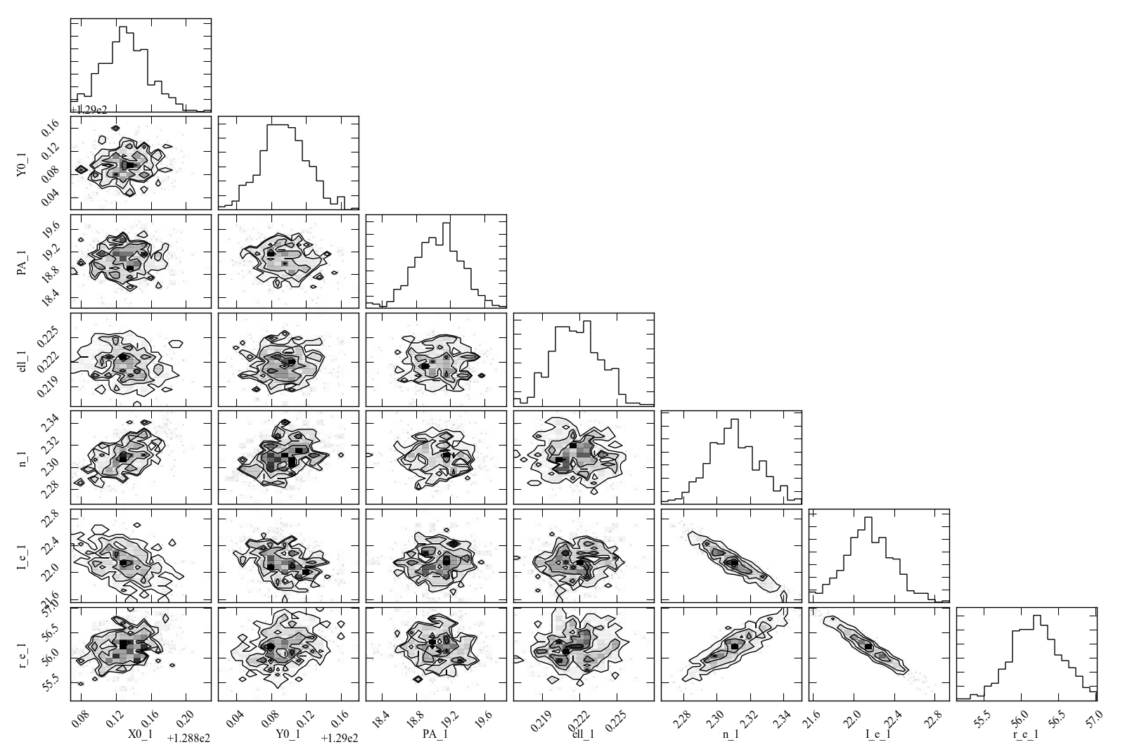
Figure 4: Scatterplot matrix of parameter values from 500 rounds of bootstrap resampling fits to the IC 3478 r-band image (Sérsic model, no PSF convolution). Note the clear correlations between the Sérsic model parameters (n, r_e, I_e).
MCMC Example
MCMC analysis uses a separate program called imfit-mcmc. You can run
it with the following command (note that it’s identical to the regular
imfit command, except for the option that specifies the root name
for output files):
imfit-mcmc ic3478rss_256.fits -c config_sersic_ic3478_256.dat
  --mask ic3478rss_256_mask.fits --gain=4.725 --readnoise=4.3
  --sky=130.14 --output=mcmc_ic3478r
Warning: this will take several minutes! (On my 2012 MacBook Pro with a quad-core Intel i7 CPU, it takes about eight or ten minutes.)
Various updates will be printed as the program runs. Once a trial
“burn-in” phase is over, imfit-mcmc will test for possible
convergence of the chains every 5,000 generations by looking at the last
half of each chain. If convergence is detected, the program will quit;
otherwise, it will quit when it reaches 100,000 generations. (These
values can be changed with command-line options.)
When it’s done, you will have seven output text files, named mcmc_ic3478r.1.txt, mcmc_ic3478r.2.txt, etc., one for each of the individual chains. (By default, the total number of chains is equal to the number of free parameters in the model.) Each is similar to the bootstrap-resampling output file in format, with one column for each parameter in the model (plus some extra bookkeeping columns that you can ignore unless you’re interested in details of the MCMC process), and one row for each generation in the chain; each chain will have several tens of thousands of generations.
The ideal thing to do is probably to take the last half of each chain and combine them all into one gigantic set of parameter values. There’s a Python function for that in python/imfit.py, which returns the same kinds of output as imfit.GetBootstrap (i.e., a list of parameter names and a 2D Numpy array). Here’s an example of using that, and then making a scatterplot matrix with the corner.py module, just as we did for the bootstrap output:
>>> import imfit, corner

>>> columnNames, allchains = imfit.MergeChains("mcmc_ic3478r",
    secondHalf=True)
>>> corner.corner(allchains, labels=columnNames)
The result is shown below.
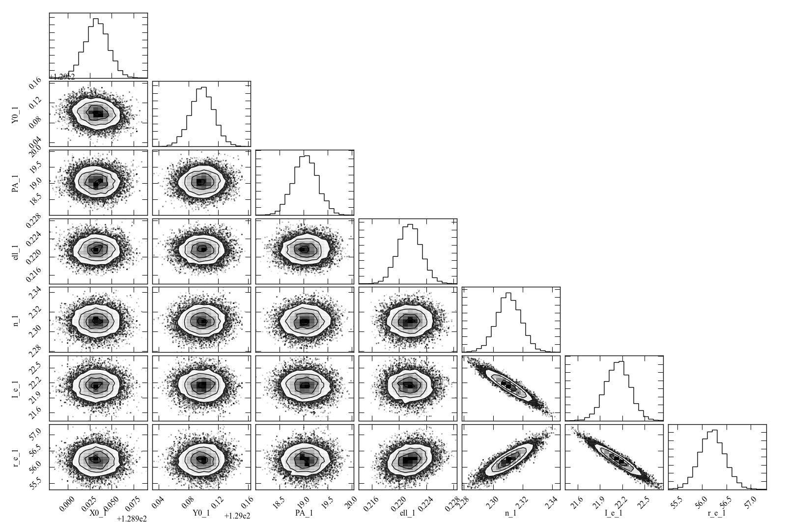
Figure 5: Scatterplot matrix of parameter values from Markov chain Monte Carlo analysis of the IC 3478 r-band image (Sérsic model, no PSF convolution). Note the strong correlations between the Sérsic model parameters (n, r_e, I_e), and the weaker correlation between r_e and ellipticity and between X0 and Y0. Since this plot is based on about 300,000 samples, it is considerably less noisy than the version based on 500 rounds of bootstrap resampling in Figure 4.